Getting started

To demonstrate a typical use case for epsf, we will reproduce results from Calissendorff et al. (2023), which presented the first Y+Y dwarf binary detection. To keep the tutorial simple, we will fit a single JWST image.

Loading the Data

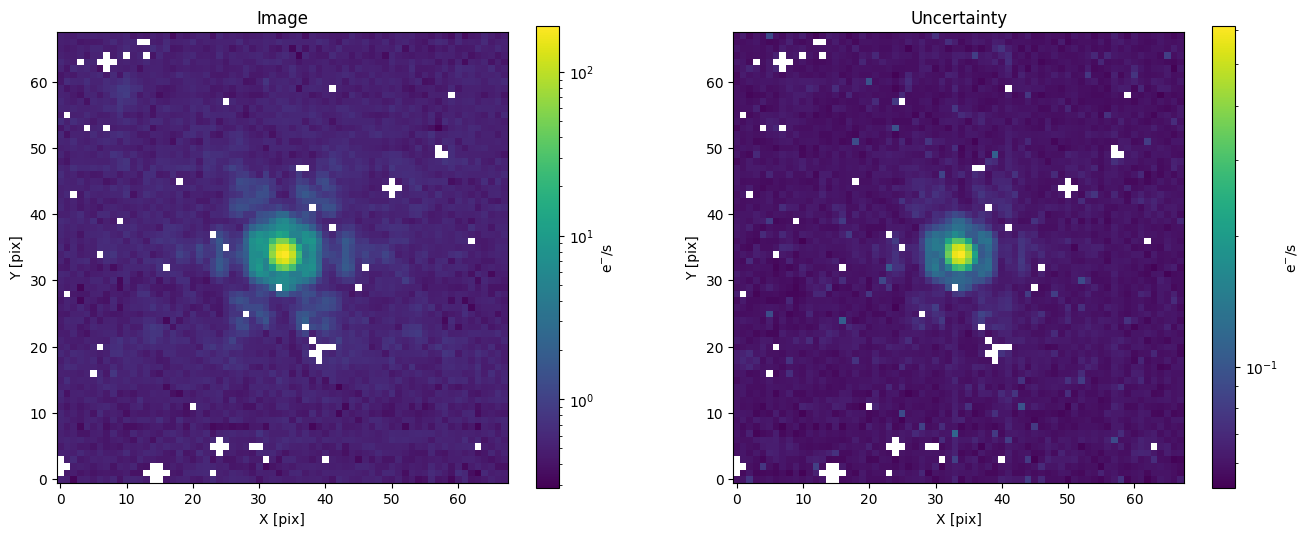
The JWST stage 2 image pipeline produces cal files, stacking all integrations in an observation. The science image is in the SCI extension and its uncertainty in the ERR extension. These are wide-field images, so we will need to extract a cutout from the image and error arrays. We know the position of the Y dwarf in this image, so we will hardcode it and take a 68x68 pixels region around it.

import numpy as np
from pathlib import Path
from astropy.io import fits
from astroquery.mast import Observations

tbl = Observations.query_criteria(
    proposal_id="02473",
    project="JWST",
    filters=["F480M", "F150W"],
)

x, y = 1281, 825
half_size = 34


img_path = Path("./data/jw02473053001_03101_00002_nrcblong_cal.fits")
img_path.parent.mkdir(exist_ok=True)
status, msg, _ = Observations.download_file(
    "mast:JWST/product/jw02473053001_03101_00002_nrcblong_cal.fits", local_path=img_path
)
hdul = fits.open(img_path)
img_full = hdul["SCI"].data
err_full = hdul["ERR"].data

crop_ind = np.s_[y - half_size : y + half_size, x - half_size : x + half_size]
img = img_full[crop_ind]
err = err_full[crop_ind]
img_pre_crop = img.copy()
err_pre_crop = err.copy()

INFO: Found cached file data/jw02473053001_03101_00002_nrcblong_cal.fits with expected size 117576000. [astroquery.query]

import matplotlib.pyplot as plt
from epsf.plot import plot_image, plot_with_diff, plot_flat_samples


fig, axs = plt.subplots(1, 2, figsize=(16, 6))
plot_image(img, ax=axs[0], color_label="e$^{-}$/s")
axs[0].set_title("Image")
plot_image(err, ax=axs[1], color_label="e$^{-}$/s")
axs[1].set_title("Uncertainty")
plt.show()

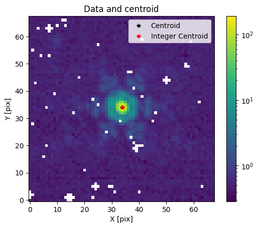
The 68x68 pixels image size we chose above was an arbitrary choice for display purposes. The effective PSF (ePSF) models from JWST1PASS are defined on an 11x11 pixels grid, so we will need to crop our image a second time. The x-y positions we used at the start were rough estimates useful only to crop the wide-field image. Let us find the centroid of the 68x68 image and then crop it to 11x11. For JWST PSFs, the centroid_quadratic function from photutils seems to do a reasonable job.

from photutils.centroids import centroid_quadratic

xy_centroid = centroid_quadratic(img, mask=np.isnan(img))
xcen_int, ycen_int = np.round(xy_centroid).astype(int)

plot_image(img)
plt.plot(*xy_centroid, "k*", label="Centroid")
plt.plot(xcen_int, ycen_int, "r*", label="Integer Centroid")
plt.title("Data and centroid")
plt.legend()
plt.show()

final_size = 11
start, end = final_size // 2, final_size // 2 + final_size % 2
x1, x2, y1, y2 = xcen_int - start, xcen_int + end, ycen_int - start, ycen_int + end
img = img_pre_crop[y1:y2, x1:x2]
err = err_pre_crop[y1:y2, x1:x2]

plot_image(img)
plt.plot(final_size // 2, final_size // 2, "r*", label="Centroid")
plt.title(f"Image cropped to {final_size}x{final_size}")
plt.show()

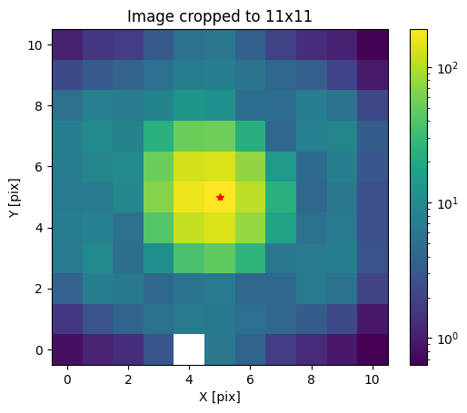
Our data is now ready to be modelled with an ePSF!

Effective PSF

Note

JWST1PASS ePSFs must first be downloaded. See the installation instructions for more detail.

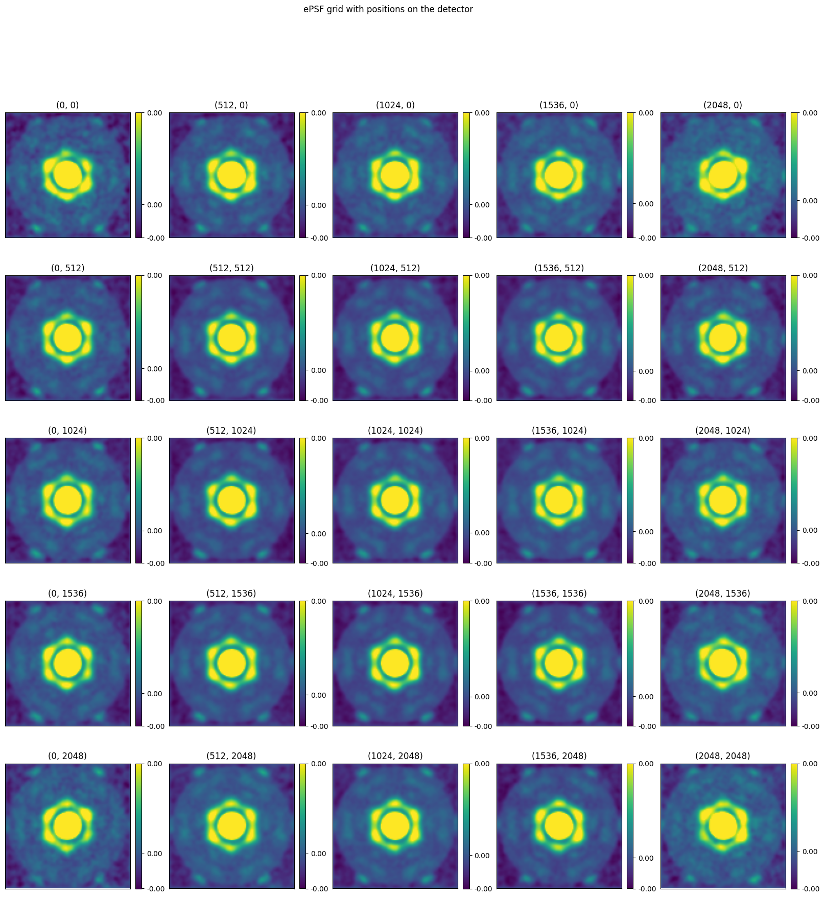
JWST1PASS ePSFs are stored as fits files with a grid of PSFs and associated detector positions stored in the header. epsf has an EPSFGrid object that stores this grid and can interpolate it to any detector position.

from epsf.grid import EPSFGrid

# There is no psf for module B so we use module A
grid = EPSFGrid.from_params("NIRCAM", "F480M", detector="NRCAL")

Before we interpolate the grid, let us look at the PSFs for all detector positions.

grid.plot()
plt.show()

To interpolate, we simply need to call the grid object with x and y detector positions, which we already have from the previous section. This will return an EPSF object, which has an array attribute storing the interpolated PSF and a spl attribute with a scipy.interpolate.RectBivariateSpline allowing us to shift the PSF to any detector position in our cutout. By default, the PSF will have a true_size of 11, meaning it can generate images of 11x11 pixels and an oversampling factor of 4, since this is what was used to generate the JWST1PASS PSFs. These two values can be changed by passing them as arguments when creating the EPSF.

psf = grid(x, y)
print(psf)

EPSF(true_size=11, oversampling=4)

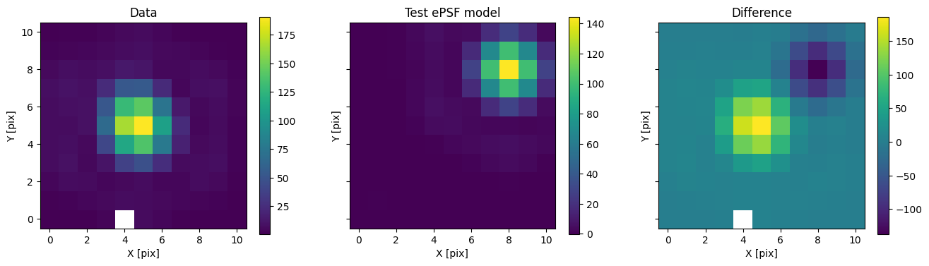
Calling the PSF object with x and y positions will generate a PSF shifted by a given amount of pixels in each direction.

test_img = 1200 * psf(3, 3)

fig, axs = plot_with_diff(img, test_img, scale="linear")
axs[0].set_title("Data")
axs[1].set_title("Test ePSF model")
axs[2].set_title("Difference")
plt.show()

Bayesian Inference

To do Bayesian inference, we could directly use the EPSF object above and write log-likelihood and prior functions to use with an MCMC or nested sampling library. However, epsf.bayes provides useful models built with simpple. That way, the likelihood and priors are already defined for us and we can use them with the sampling library of our choice.

Single model

Let us first define a model for a single source. We include a constant background term as well as a white noise term added in quadrature with our uncertainties.

We will use the UltraNest library to generate posterior samples and estimate the Bayesian evidence.

import simpple.distributions as sdist
from epsf.bayes import SingleModel

parameters = {
    "x0": sdist.Uniform(-1.5, 1.5),
    "y0": sdist.Uniform(-1.5, 1.5),
    "flux": sdist.LogUniform(1e-5, 5000),
    "bkg": sdist.Uniform(-100, 100),
    "sigma": sdist.LogUniform(1e-5, 100),
}
model = SingleModel(parameters, psf)

from ultranest import ReactiveNestedSampler

sampler = ReactiveNestedSampler(
    model.keys(), lambda p: model.log_likelihood(p, img, err), model.prior_transform
)
sampler.run(show_status=False);

[ultranest] Sampling 400 live points from prior ...

[ultranest] Explored until L=-3e+02  
[ultranest] Likelihood function evaluations: 35558
[ultranest]   logZ = -332.9 +- 0.1992
[ultranest] Effective samples strategy satisfied (ESS = 2373.5, need >400)
[ultranest] Posterior uncertainty strategy is satisfied (KL: 0.45+-0.05 nat, need <0.50 nat)
[ultranest] Evidency uncertainty strategy is satisfied (dlogz=0.20, need <0.5)
[ultranest]   logZ error budget: single: 0.25 bs:0.20 tail:0.01 total:0.20 required:<0.50
[ultranest] done iterating.

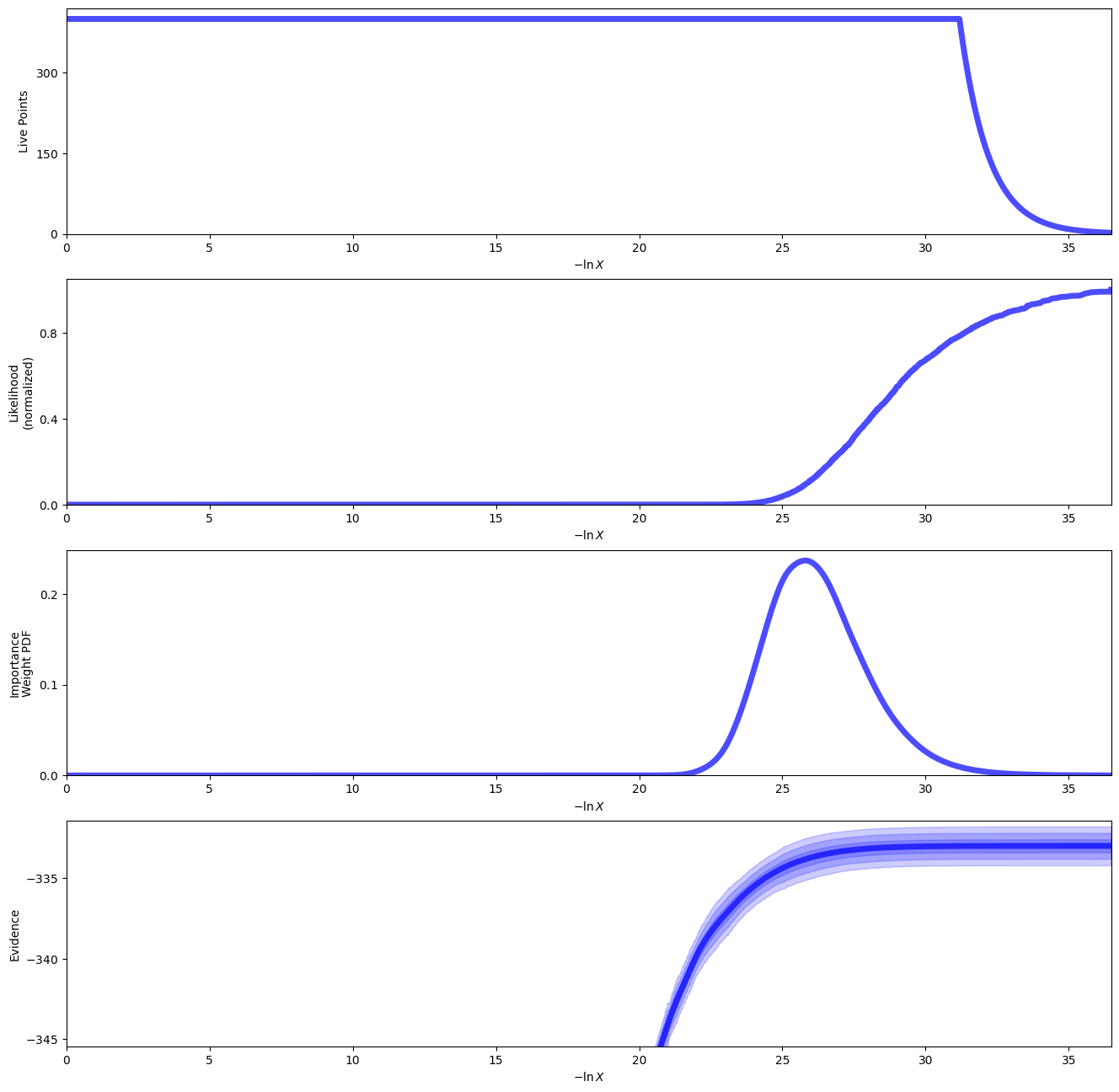
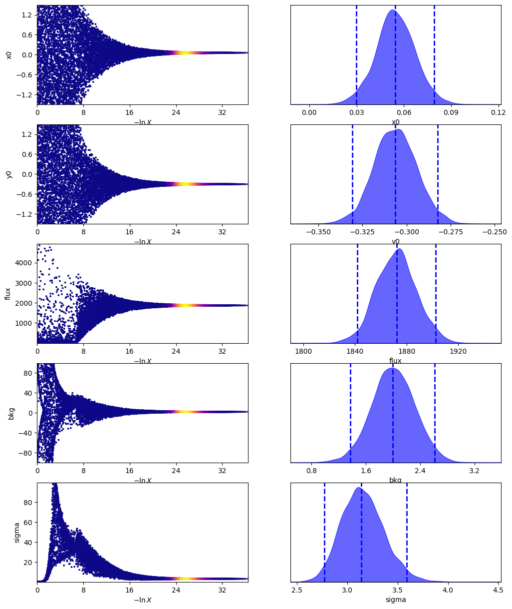
sampler.plot()
plt.show()

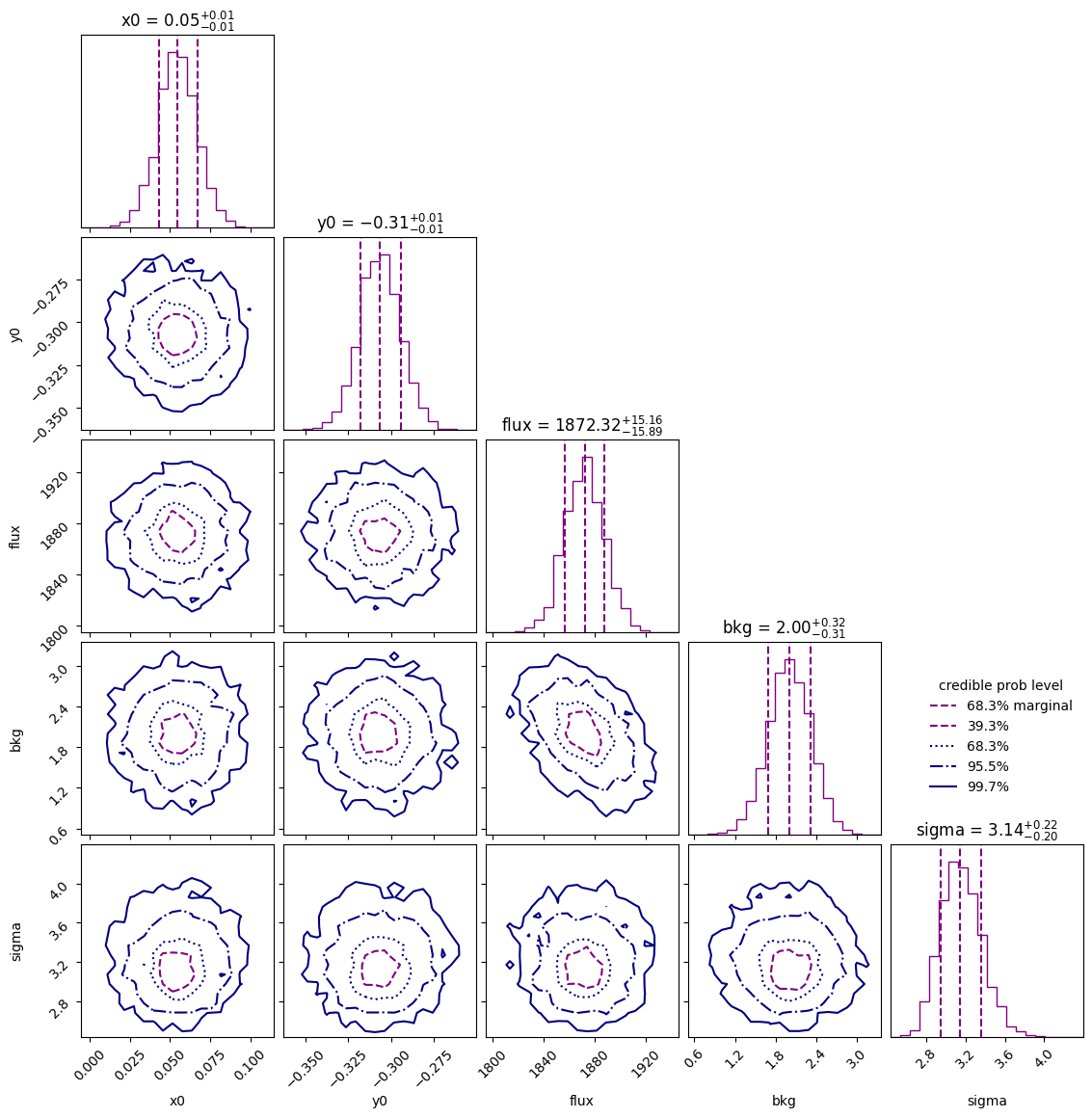
We can then use the posterior median to compare the model with the data.

med_p = dict(
    zip(
        model.keys(),
        sampler.results["posterior"]["median"],
    )
)
med_mod = model.forward(med_p)

fig, axs = plot_with_diff(img, med_mod, scale="linear")
axs[0].set_title("Data")
axs[1].set_title("Median model")
axs[2].set_title("Difference")
plt.show()

It is also useful to visualize posterior samples of the forward model compared to the data. However, this is a bit cumbersome to display for images. We would need a grid of samples and a grid of residuals. As an alternative, we will flatten the image and compare the pixel values with predictions from the model on a 1D plot.

plot_flat_samples(img, err, model.get_posterior_pred(sampler.results["samples"].T, 100))
plt.show()

Binary model

We will now repeat the same steps as above, but with a binary model.

from epsf.bayes import BinaryModel

parameters = {
    "x0": sdist.Uniform(-1.5, 1.5),
    "y0": sdist.Uniform(-1.5, 1.5),
    "flux": sdist.LogUniform(1e-5, 5000),
    "bkg": sdist.Uniform(-100, 100),
    "sep": sdist.Uniform(0.5, 5),
    "pa": sdist.Uniform(0, 360),
    "cr": sdist.LogUniform(1e-4, 1.0),
    "sigma": sdist.LogUniform(1e-4, 100.0),
}
model_binary = BinaryModel(parameters, psf)

Since we have more parameters, UltraNest will struggle to generate valid samples in a high-dimensional space. Instead of region sampling, we add a stepsampler to our nested sampler. This enables a more efficient exploration of parameter space.

from ultranest.stepsampler import SliceSampler, generate_mixture_random_direction

wrapped_params = [pname == "pa" for pname in model_binary.keys()]
nsteps = len(model.keys()) * 2
sampler_binary = ReactiveNestedSampler(
    model_binary.keys(),
    lambda p: model_binary.log_likelihood(p, img, err),
    model_binary.prior_transform,
    wrapped_params=wrapped_params,
)
sampler_binary.stepsampler = SliceSampler(
    nsteps=nsteps,
    generate_direction=generate_mixture_random_direction,
)

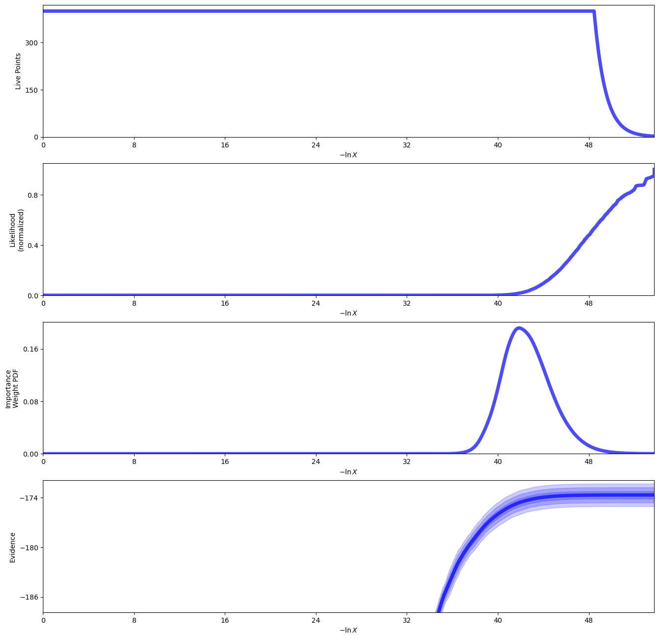
sampler_binary.run(show_status=True);

[ultranest] Sampling 400 live points from prior ...

[ultranest] Explored until L=-1e+02  .37 [-130.0117..-130.0115]*| it/evals=19379/751016 eff=2.5817% N=400  400   0 00 0 
[ultranest] Likelihood function evaluations: 751359
[ultranest]   logZ = -173.7 +- 0.2281
[ultranest] Effective samples strategy satisfied (ESS = 2948.1, need >400)
[ultranest] Posterior uncertainty strategy is satisfied (KL: 0.45+-0.05 nat, need <0.50 nat)
[ultranest] Evidency uncertainty strategy wants 398 minimum live points (dlogz from 0.19 to 0.57, need <0.5)
[ultranest]   logZ error budget: single: 0.32 bs:0.23 tail:0.01 total:0.23 required:<0.50
[ultranest] done iterating.

sampler_binary.plot()
plt.show()

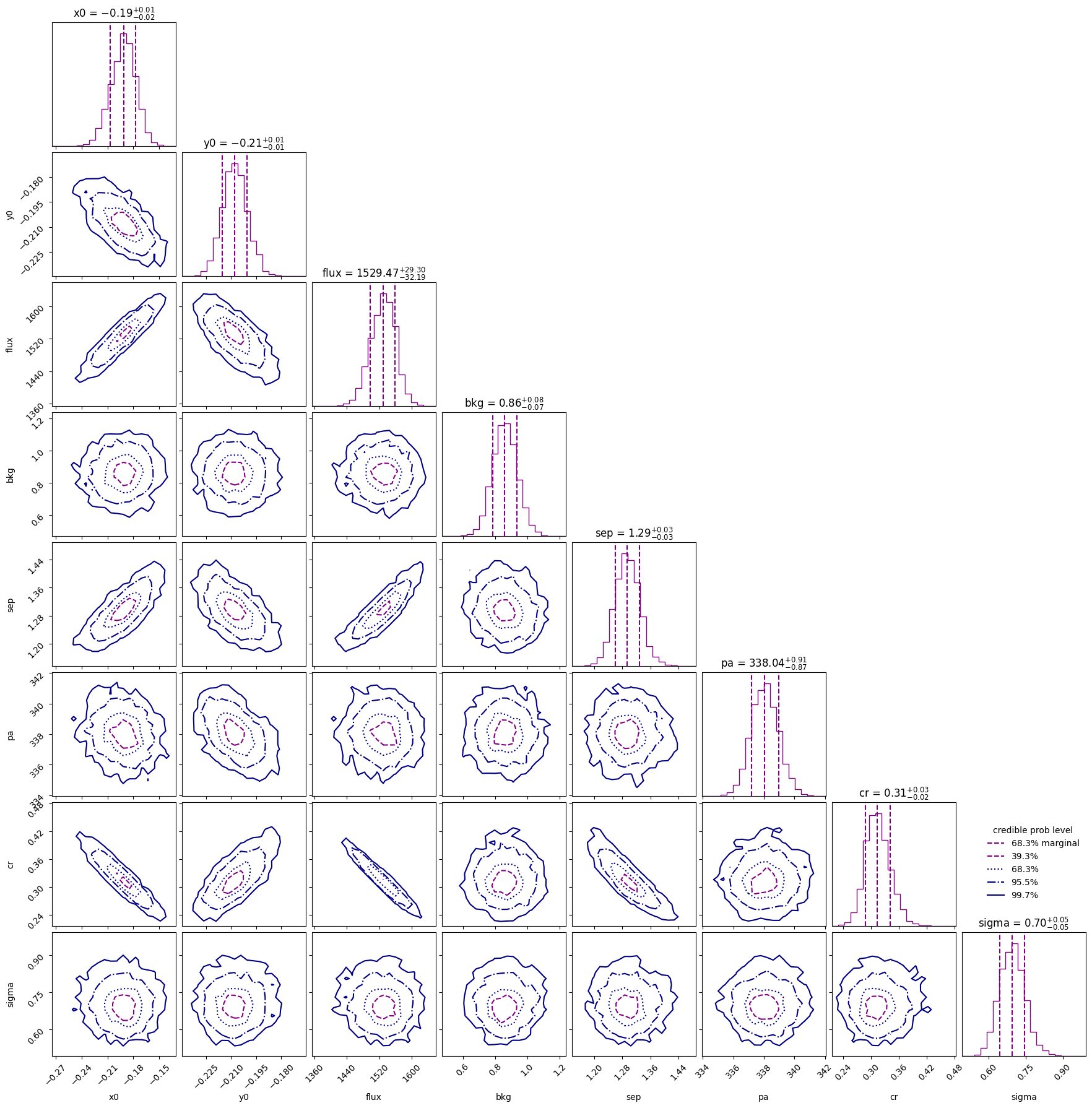
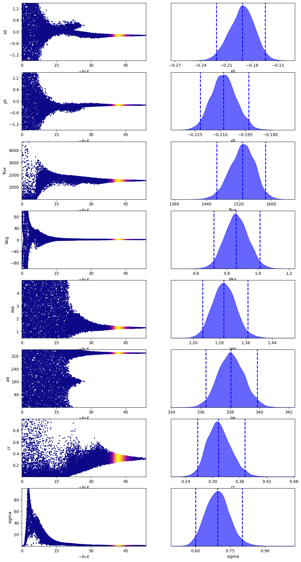
One thing to note here is that the contrast is different from Calissendorff et al. (2023). This is most likely due to the fact they used a custom ePSF model instead of one from JWST1PASS. We will look into this in a future release.

med_p = dict(
    zip(
        model_binary.keys(),
        sampler_binary.results["posterior"]["median"],
    )
)
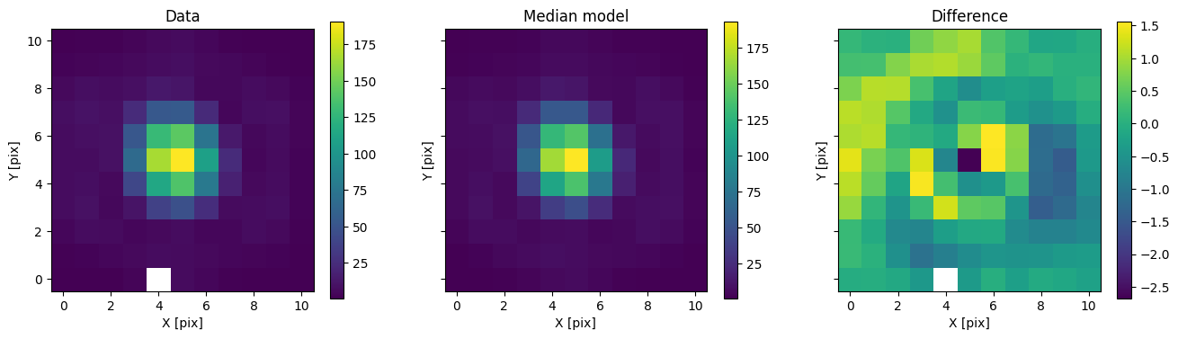
med_mod = model_binary.forward(med_p)

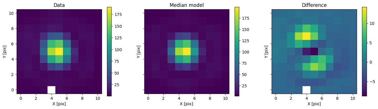
fig, axs = plot_with_diff(img, med_mod, scale="linear")
axs[0].set_title("Data")
axs[1].set_title("Median model")
axs[2].set_title("Difference")
plt.show()

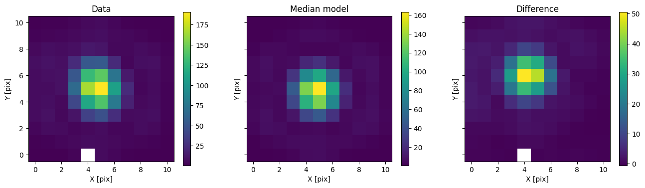
In addition to comparing the median binary model, we can subtract only the primary to see the companion pop up.

med_mod_primary = model.forward(med_p)
fig, axs = plot_with_diff(img, med_mod_primary, scale="linear")
axs[0].set_title("Data")
axs[1].set_title("Median model")
axs[2].set_title("Difference")
plt.show()

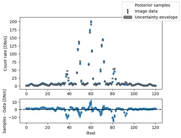
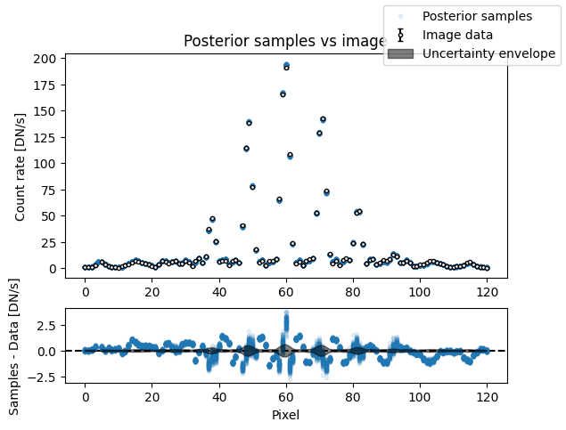
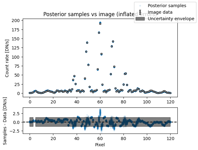
fig, axs = plot_flat_samples(
    img, err, model_binary.get_posterior_pred(sampler_binary.results["samples"].T, 100)
)
axs[0].set_title("Posterior samples vs image")
plt.show()

median_sigma = sampler_binary.results["posterior"]["median"][
    model.keys().index("sigma")
]
fig, axs = plot_flat_samples(
    img,
    np.sqrt(err**2 + median_sigma**2),
    model_binary.get_posterior_pred(sampler_binary.results["samples"].T, 100),
)
axs[0].set_title("Posterior samples vs image (inflated errors)")
plt.show()

Model comparison

Let us now compare the single and binary models using the Bayes factor.

print(f"lnZ single: {sampler.results['logz']:.2f} +/- {sampler.results['logzerr']:.2f}")
print(
    f"lnZ binary: {sampler_binary.results['logz']:.2f} +/- {sampler_binary.results['logzerr']:.2f}"
)
lnK = sampler_binary.results["logz"] - sampler.results["logz"]
lnK_err = np.sqrt(
    sampler.results["logzerr"] ** 2 + sampler_binary.results["logzerr"] ** 2
)
print(f"lnK binary - single: {lnK:.2f} +/- {lnK_err:.2f}")

lnZ single: -332.98 +/- 0.40
lnZ binary: -173.69 +/- 0.35
lnK binary - single: 159.29 +/- 0.53

As expected, the binary model is overwhelmingly favored by the data.