ePSF modelling of multiple images#
As in the Getting Started, we will replicate results from Calissendorff et al. (2023), mainly because this is the dataset I have in hand as of writing this.
This time, instead of fitting a single image, we will demonstrate how epsf can fit multiple images of the same source simultaneously.
Loading images#
from pathlib import Path
from astroquery.mast import Observations

img_dir = Path("./data")
img_dir.mkdir(exist_ok=True)
img_paths = []
for i in range(1, 6):
    filename = f"jw02473053001_03101_0000{i}_nrcblong_cal.fits"
    img_path = img_dir / filename
    status, msg, _ = Observations.download_file(
        f"mast:JWST/product/{filename}", local_path=img_path
    )
    img_paths.append(img_path)
nimg = len(img_paths)
INFO: Found cached file data/jw02473053001_03101_00001_nrcblong_cal.fits with expected size 117576000. [astroquery.query]
INFO: Found cached file data/jw02473053001_03101_00002_nrcblong_cal.fits with expected size 117576000. [astroquery.query]
INFO: Found cached file data/jw02473053001_03101_00003_nrcblong_cal.fits with expected size 117576000. [astroquery.query]
INFO: Found cached file data/jw02473053001_03101_00004_nrcblong_cal.fits with expected size 117576000. [astroquery.query]
INFO: Found cached file data/jw02473053001_03101_00005_nrcblong_cal.fits with expected size 117576000. [astroquery.query]
import numpy as np
import matplotlib.pyplot as plt

import epsf.utils as ut
from epsf.plot import plot_mosaic, plot_with_diff, plot_flat_samples

# The dithers could have different positions so let us make this generic
pos_arr = np.array([[1281, 825]] * nimg)
half_size = 34
final_size = 11

img_arr = np.empty((nimg, final_size, final_size))
err_arr = np.empty((nimg, final_size, final_size))
for i, img_path in enumerate(img_paths):
    img_arr[i], err_arr[i] = ut.open_jwst_image(
        img_path,
        pos_cut=pos_arr[i],
        half_size_cut=half_size,
        final_size=final_size,
        recenter=True,
    )
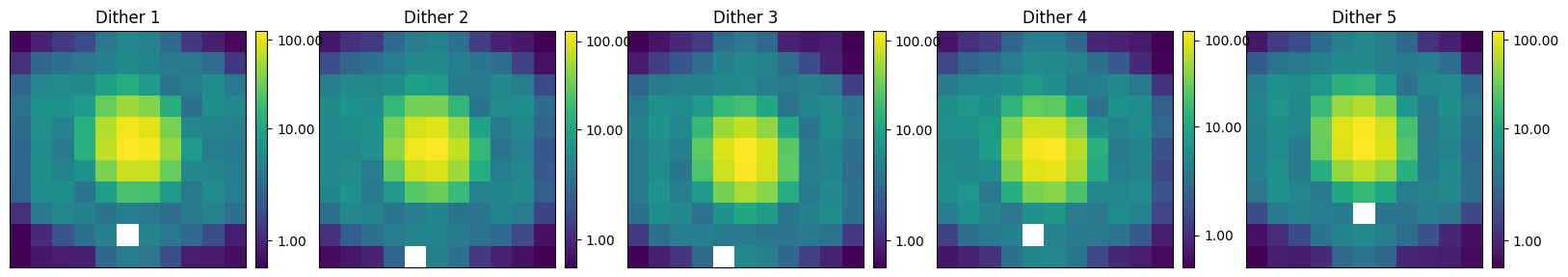
titles = [f"Dither {i}" for i in range(1, nimg + 1)]
plot_mosaic(img_arr, nrows=1, ncols=nimg, titles=titles)
plt.show()
Note
JWST1PASS ePSFs must first be downloaded. See the installation instructions for more detail.
from epsf.grid import EPSFGrid

# There is no PSF for module B so we use module A
grid = EPSFGrid.from_params("NIRCAM", "F480M", detector="NRCAL")
psf_list = [grid(*pos) for pos in pos_arr]
Single#
import simpple.distributions as sdist
from epsf.bayes import SingleModelMulti

x_params = {f"x0{i}": sdist.Uniform(-1.5, 1.5) for i in range(nimg)}
y_params = {f"y0{i}": sdist.Uniform(-1.5, 1.5) for i in range(nimg)}
parameters = (
    {
        "flux": sdist.LogUniform(1e-5, 5000),
        "bkg": sdist.Uniform(-100, 100),
        "sigma": sdist.LogUniform(1e-5, 100),
    }
    | x_params
    | y_params
)
model = SingleModelMulti(parameters, psf_list)
from ultranest import ReactiveNestedSampler

sampler = ReactiveNestedSampler(
    model.keys(),
    lambda p: model.log_likelihood(p, img_arr, err_arr),
    model.prior_transform,
)
sampler.run(show_status=False);
[ultranest] Sampling 400 live points from prior ...
[ultranest] Explored until L=-1e+03
[ultranest] Likelihood function evaluations: 233044
[ultranest]   logZ = -1361 +- 0.2023
[ultranest] Effective samples strategy satisfied (ESS = 3677.8, need >400)
[ultranest] Posterior uncertainty strategy is satisfied (KL: 0.45+-0.07 nat, need <0.50 nat)
[ultranest] Evidency uncertainty strategy wants 398 minimum live points (dlogz from 0.15 to 0.51, need <0.5)
[ultranest]   logZ error budget: single: 0.39 bs:0.20 tail:0.01 total:0.20 required:<0.50
[ultranest] done iterating.
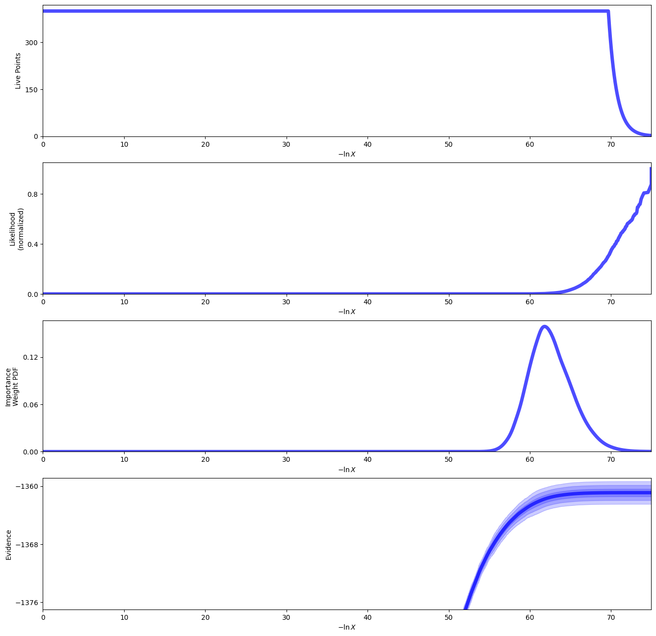
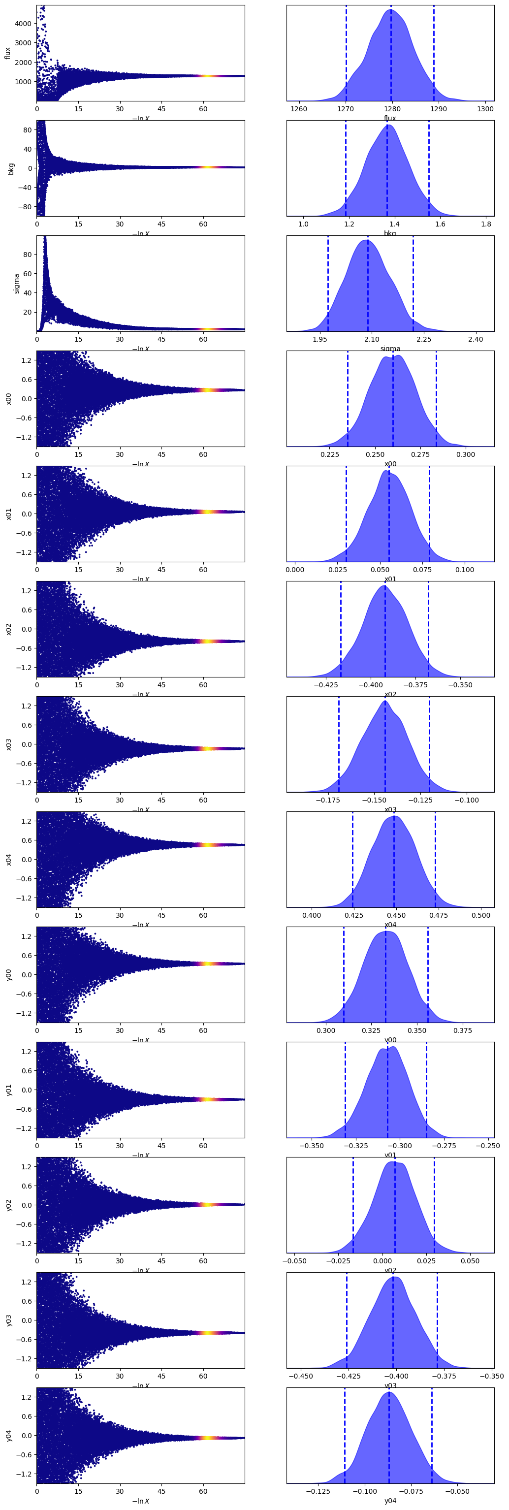
sampler.plot()
plt.show()
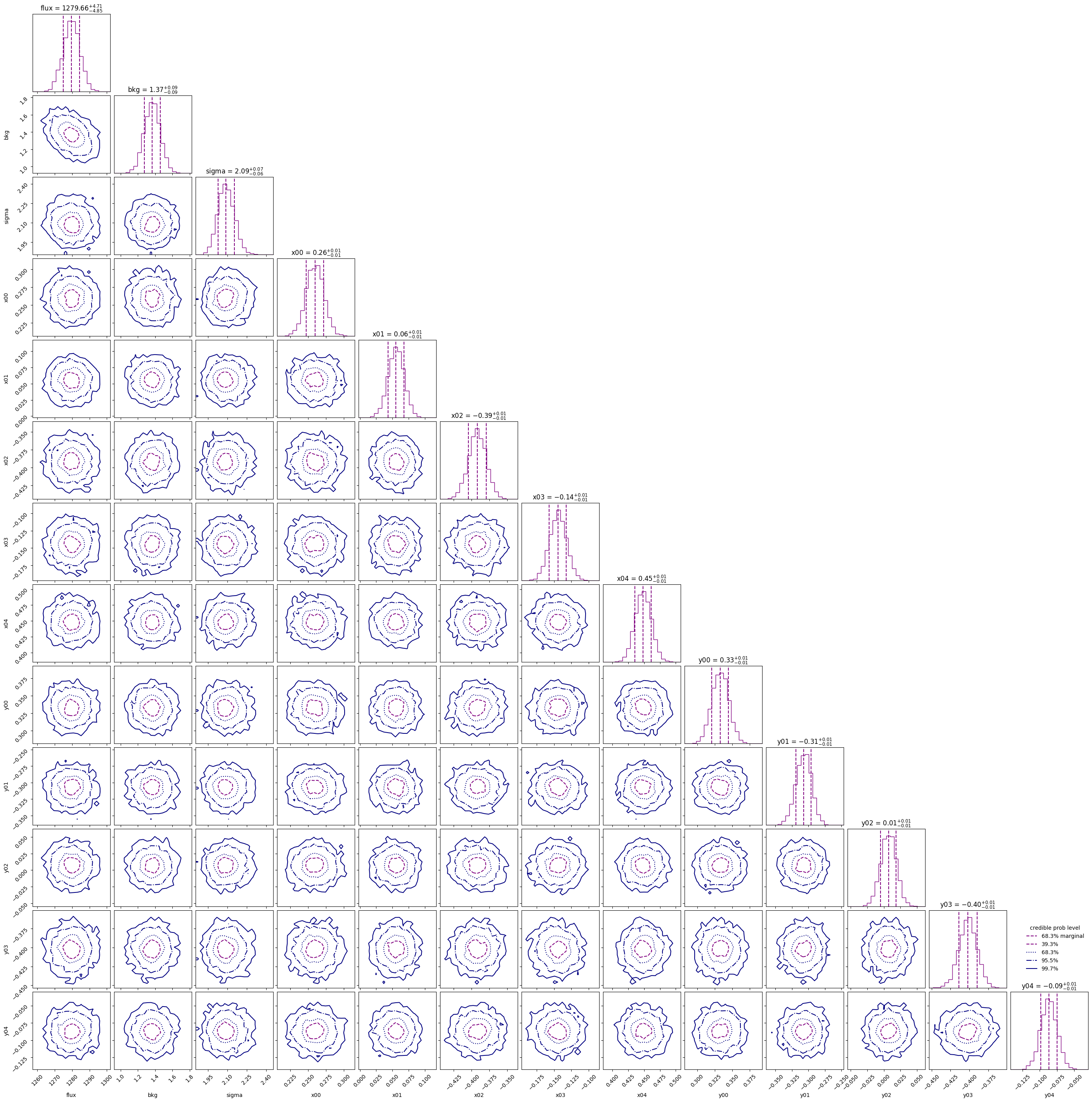
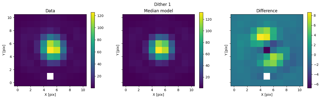
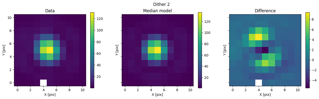
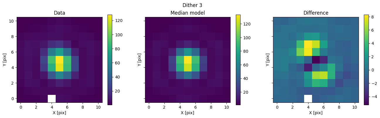
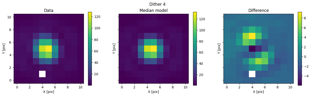
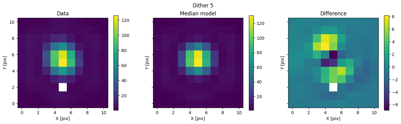
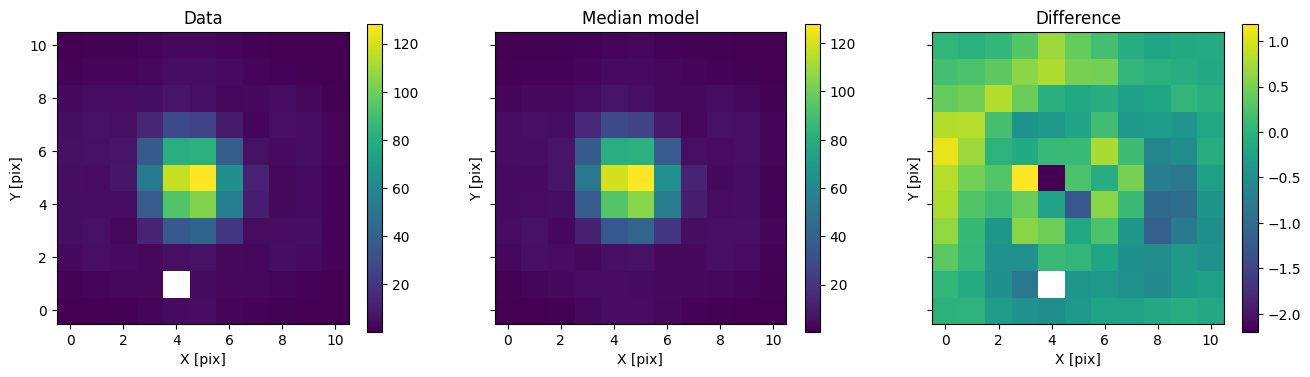
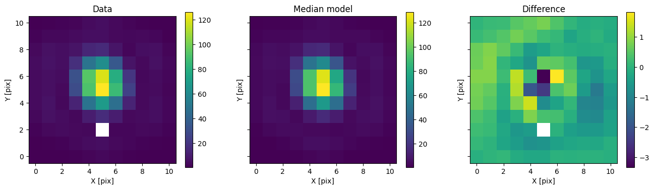
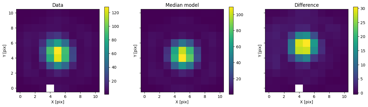
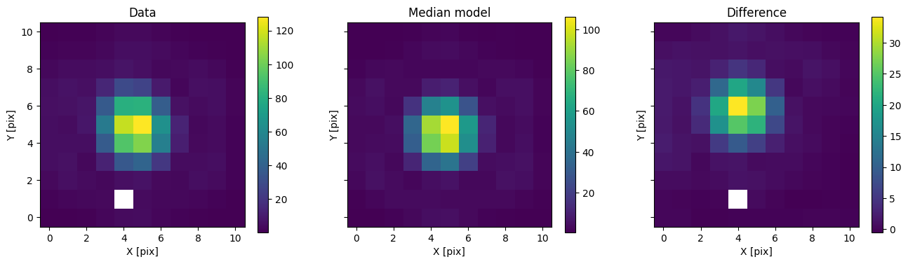
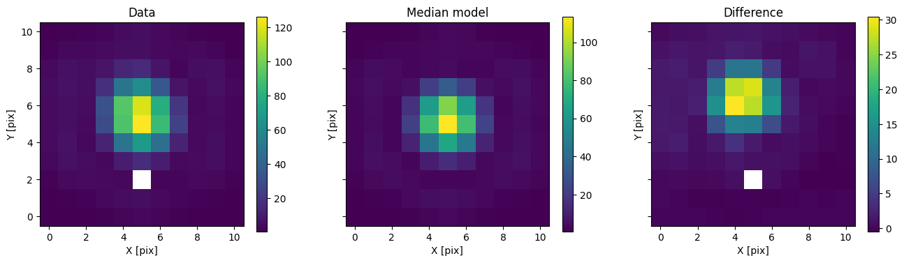
We can then use the posterior median to compare the model with the data.
med_p = dict(
    zip(
        model.keys(),
        sampler.results["posterior"]["median"],
    )
)
med_mod = model.forward(med_p)

for i in range(nimg):
    fig, axs = plot_with_diff(img_arr[i], med_mod[i], scale="linear")
    axs[0].set_title("Data")
    axs[1].set_title("Median model")
    axs[2].set_title("Difference")
    fig.suptitle(f"Dither {i + 1}")
    plt.show()
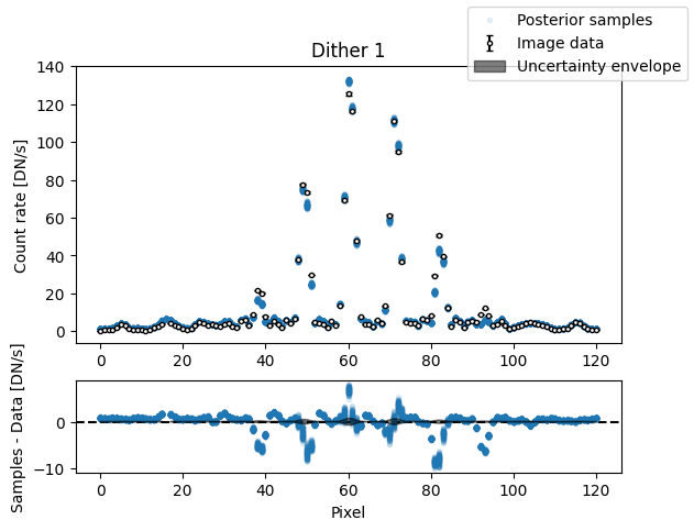
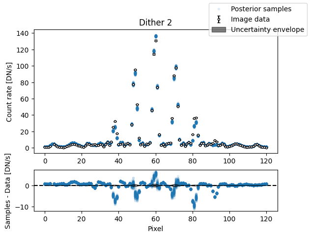
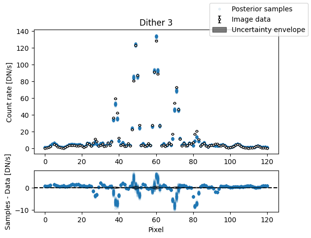
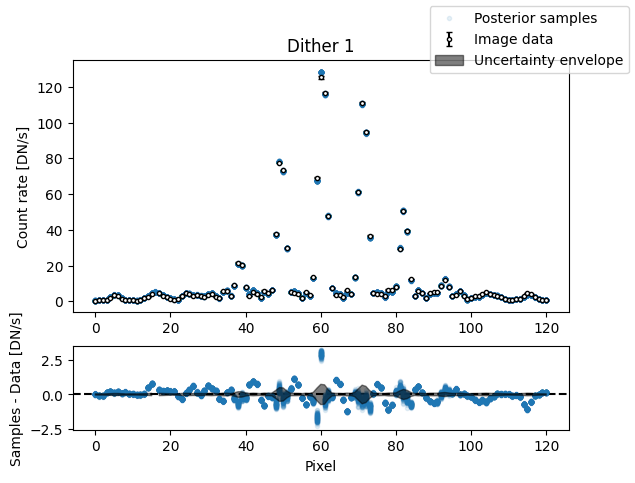
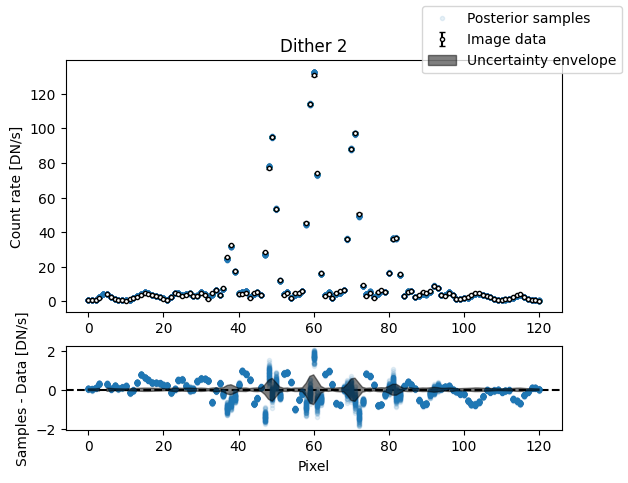
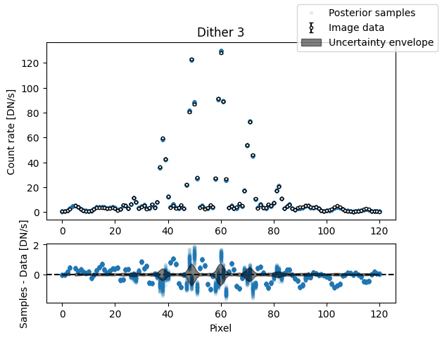
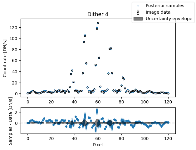
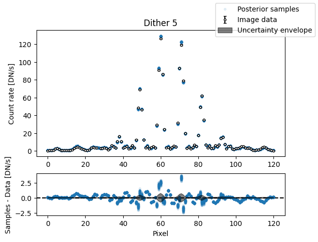
img_samples = model.get_posterior_pred(sampler.results["samples"].T, 100)
for i in range(nimg):
    fig, axs = plot_flat_samples(img_arr[i], err_arr[i], img_samples[:, i])
    axs[0].set_title(f"Dither {i + 1}")
plt.show()
Binary model#
We will now repeat the same steps as above, but with a binary model.
from epsf.bayes import BinaryModelMulti

x_params = {f"x0{i}": sdist.Uniform(-1.5, 1.5) for i in range(nimg)}
y_params = {f"y0{i}": sdist.Uniform(-1.5, 1.5) for i in range(nimg)}
parameters = (
    {
        "flux": sdist.LogUniform(1e-5, 5000),
        "sep": sdist.Uniform(0.5, 5),
        "pa": sdist.Uniform(0, 360),
        "cr": sdist.LogUniform(1e-4, 1.0),
        "bkg": sdist.Uniform(-100, 100),
        "sigma": sdist.LogUniform(1e-5, 100),
    }
    | x_params
    | y_params
)
model_binary = BinaryModelMulti(parameters, psf_list)
Since we have more parameters, UltraNest will struggle to generate valid samples in a high-dimensional space. Instead of region sampling, we add a stepsampler to our nested sampler. This enables a more efficient exploration of parameter space.
from ultranest.stepsampler import SliceSampler, generate_mixture_random_direction
nsteps = len(model.keys()) * 2
wrapped_params = [pname == "pa" for pname in model_binary.keys()]
sampler_binary = ReactiveNestedSampler(
model_binary.keys(),
lambda p: model_binary.log_likelihood(p, img_arr, err_arr),
model_binary.prior_transform,
wrapped_params=wrapped_params,
)
sampler_binary.stepsampler = SliceSampler(
nsteps=nsteps,
generate_direction=generate_mixture_random_direction,
)
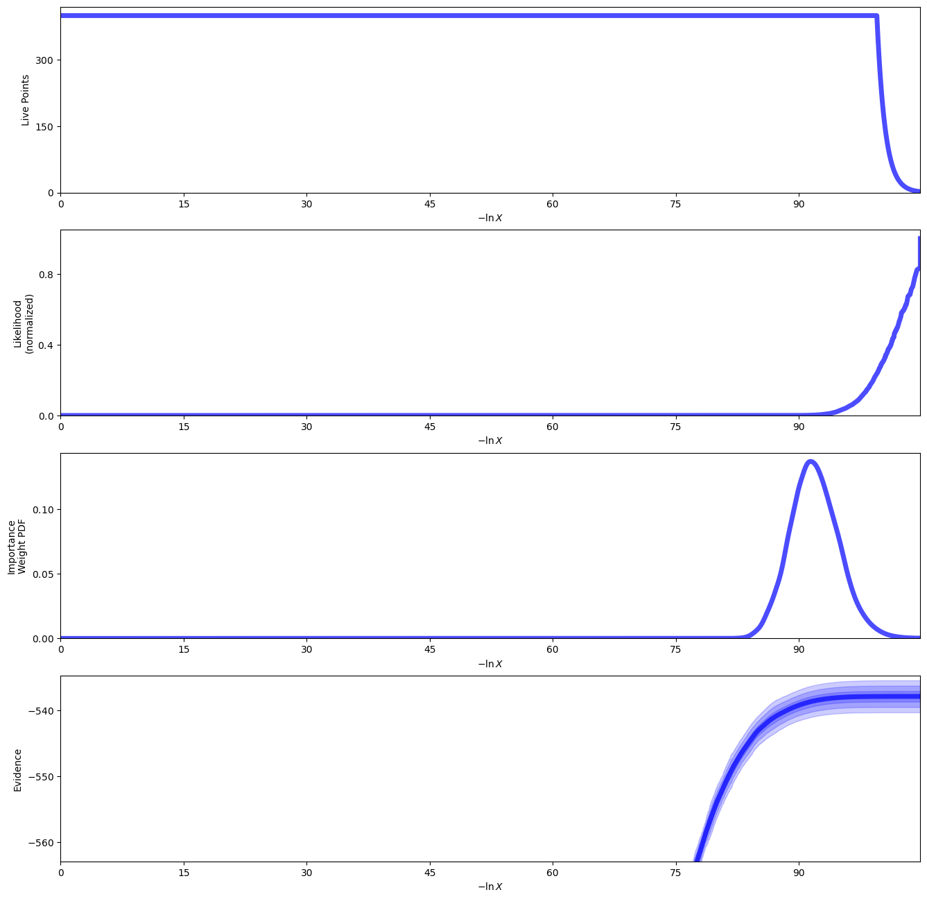
sampler_binary.run(show_status=False);
[ultranest] Sampling 400 live points from prior ...
[ultranest] Explored until L=-4e+02
[ultranest] Likelihood function evaluations: 4142492
[ultranest]   logZ = -537.8 +- 0.2651
[ultranest] Effective samples strategy satisfied (ESS = 4150.9, need >400)
[ultranest] Posterior uncertainty strategy is satisfied (KL: 0.46+-0.06 nat, need <0.50 nat)
[ultranest] Evidency uncertainty strategy wants 398 minimum live points (dlogz from 0.22 to 0.66, need <0.5)
[ultranest]   logZ error budget: single: 0.47 bs:0.27 tail:0.01 total:0.27 required:<0.50
[ultranest] done iterating.
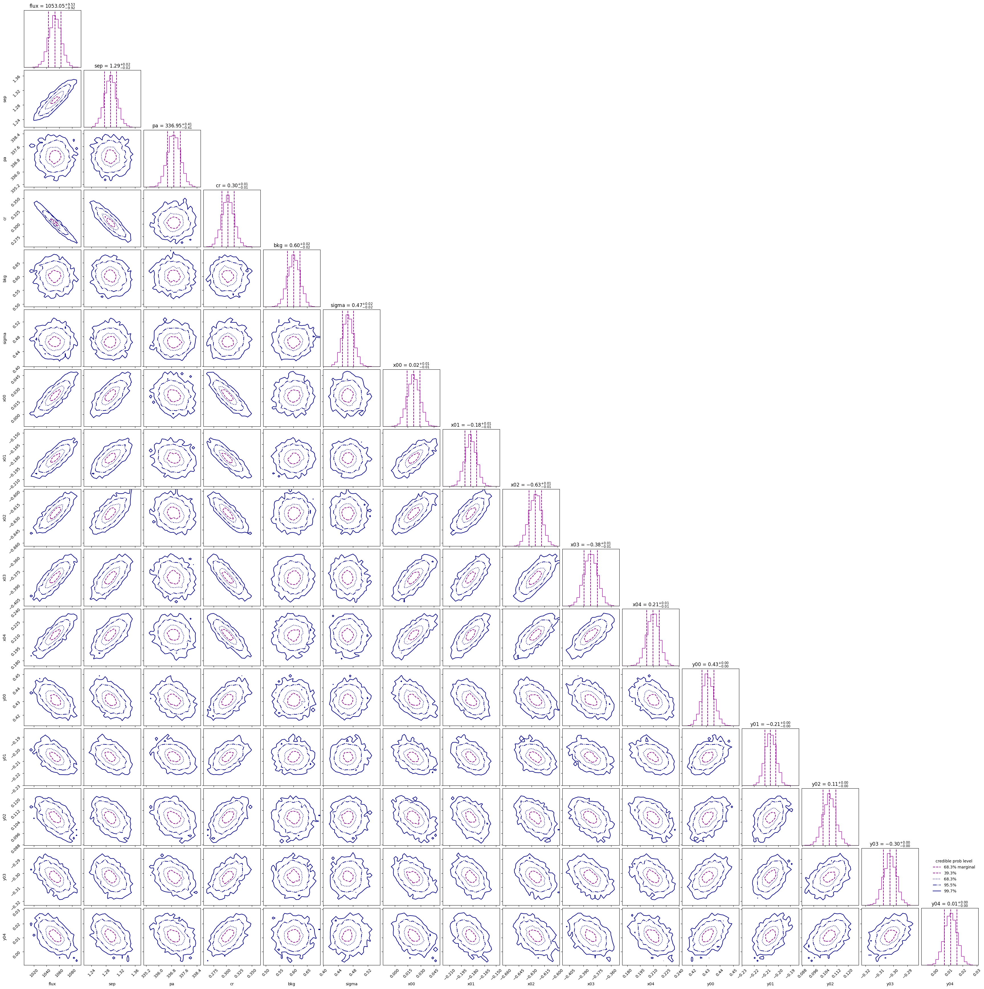
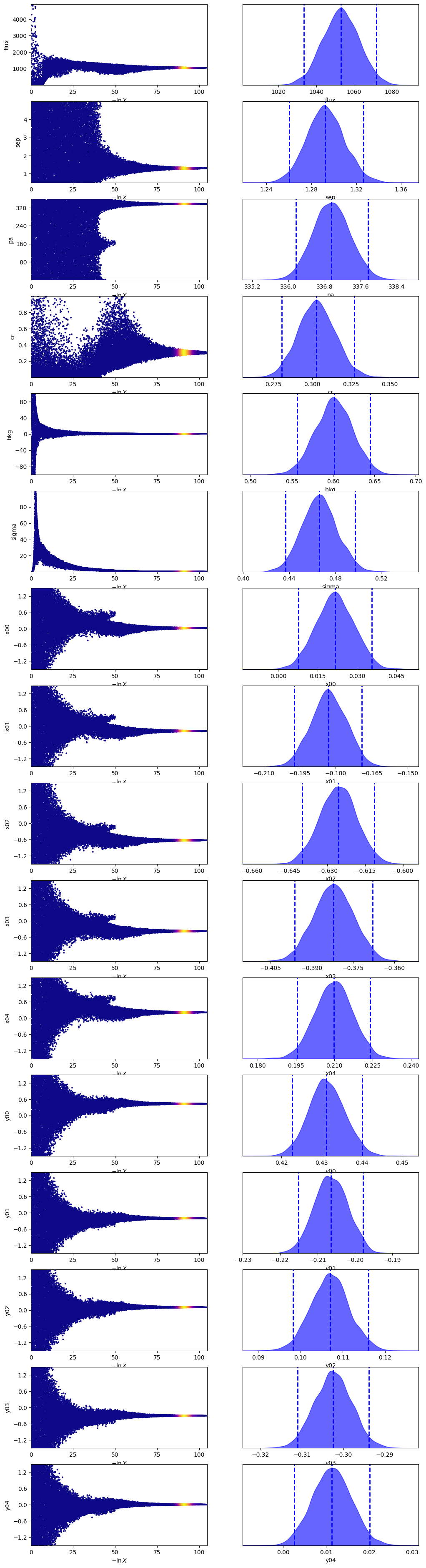
sampler_binary.plot()
plt.show()
med_p = dict(
zip(
model_binary.keys(),
sampler_binary.results["posterior"]["median"],
)
)
med_mod = model_binary.forward(med_p)
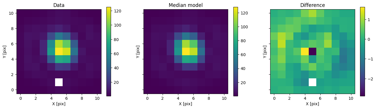
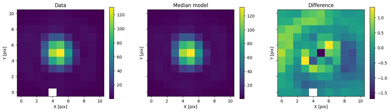
for i in range(nimg):
fig, axs = plot_with_diff(img_arr[i], med_mod[i], scale="linear")
axs[0].set_title("Data")
axs[1].set_title("Median model")
axs[2].set_title("Difference")
plt.show()
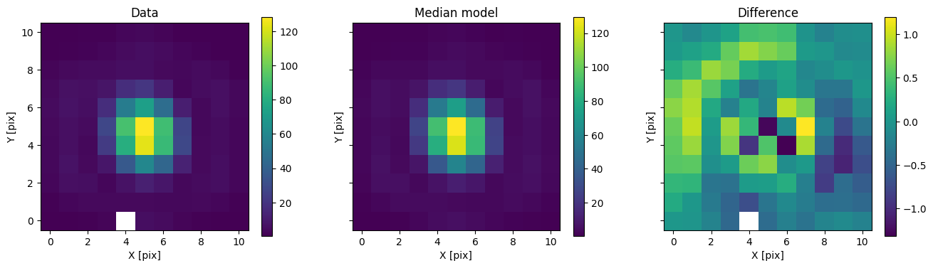
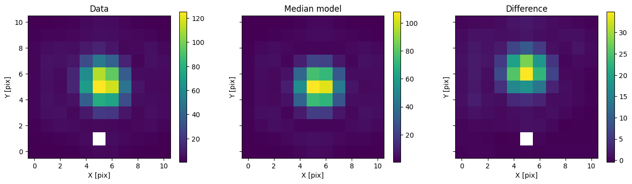
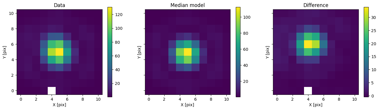
In addition to comparing the median binary model, we can subtract only the primary to see the companion pop up.
med_mod_primary = model.forward(med_p)
for i in range(nimg):
    fig, axs = plot_with_diff(img_arr[i], med_mod_primary[i], scale="linear")
    axs[0].set_title("Data")
    axs[1].set_title("Median model")
    axs[2].set_title("Difference")
    plt.show()
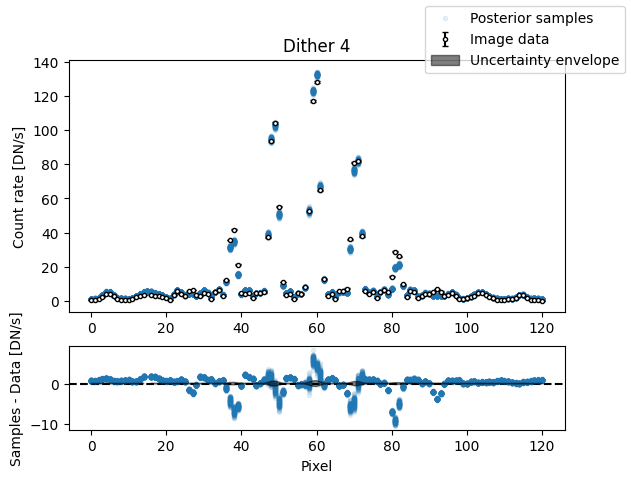
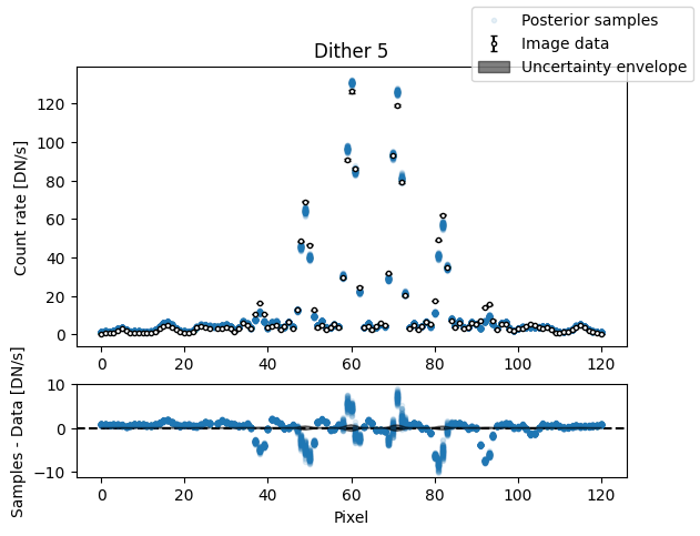
img_samples = model_binary.get_posterior_pred(sampler_binary.results["samples"].T, 100)
for i in range(nimg):
    fig, axs = plot_flat_samples(img_arr[i], err_arr[i], img_samples[:, i])
    axs[0].set_title(f"Dither {i + 1}")
plt.show()
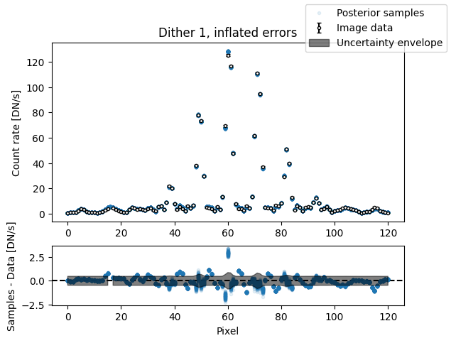
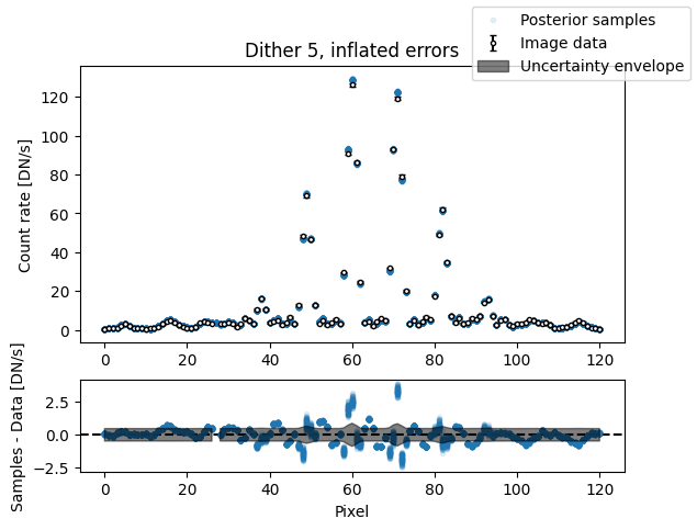
img_samples = model_binary.get_posterior_pred(sampler_binary.results["samples"].T, 100)
median_sigma = sampler_binary.results["posterior"]["median"][
    model_binary.keys().index("sigma")
]
inflated_err = np.sqrt(err_arr**2 + median_sigma**2)
for i in range(nimg):
    fig, axs = plot_flat_samples(img_arr[i], inflated_err[i], img_samples[:, i])
    axs[0].set_title(f"Dither {i + 1}, inflated errors")
plt.show()
Model comparison#
Let us now compare the single and binary models using the Bayes factor.
print(f"lnZ single {sampler.results['logz']:.2f} +/- {sampler.results['logzerr']:.2f}")
print(
    f"lnZ binary {sampler_binary.results['logz']:.2f} +/- {sampler_binary.results['logzerr']:.2f}"
)
lnK = sampler_binary.results["logz"] - sampler.results["logz"]
lnK_err = np.sqrt(
    sampler.results["logzerr"] ** 2 + sampler_binary.results["logzerr"] ** 2
)
print(f"lnK binary - single {lnK:.2f} +/- {lnK_err:.2f}")
lnZ single -1360.90 +/- 0.41
lnZ binary -537.86 +/- 0.66
lnK binary - single 823.04 +/- 0.78
As expected, the binary model is overwhelmingly favored by the data.